Strain-Displacement Relations

Notation. It is convenient to use the index notation. Co-ordinate axes $x,\ y$ and z will henceforth be denoted by $x_1,\ x_2$and x₃ respectively. Co-ordinates of a point in the reference configuration will be denoted by X₁,X₂,X₃, and those in the present configuration by x₁,x₂,x₃. Components of a vector A will be denoted by A₁,A₂,A₃ rather than by $A_x,\ A_y$ and A_z. Thus

$$\mathbf{A} = A_1\hat i_1 + A_2\hat i_2 + A_3\hat i_3\tag{5.1}$$ (5.1)

where $\hat i_1,\ \hat i_2$ and $\hat i_3$ are unit vectors along $x_1,\ x_2$ and x₃ axes respectively. We shall also adopt the following summation convention: a repeated index implies summation over the range of the index. That is, an index appearing twice (not more) in a term implies the sum of terms. Thus the inner product between two vectors A and B can be written as

$$\mathbf{A}\cdot\mathbf{B} = A_1B_1 + A_2B_2 + A_3B_3 = A_jB_j = A_\ell B_\ell . \tag{5.2}$$ (5.2)

Note that the repeated index is dummy. Recall that

$$\int^1_0 \sin\theta d\theta = \int^1_0 \sin ydy = \int^1_0\sin xdx.\tag{5.3}$$ (5.3)

Thus, the repeated index in (5.2) plays the same role as the variable of integration does in (5.3).

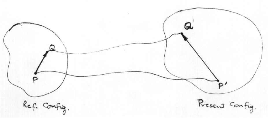
Due to the application of loads to the body, let points P(X₁,X₂,X₃) and Q(X₁ + dX₁,X₂ + dX₂,X₃ + dX₃) in the reference configuration move to places $P^\prime (x_1,x_2,x_3)$ and $Q^\prime (x_1 + dx_1,x_2 + dx_2,x_3 + dx_3)$ in the present configuration. We assume that different material particles always occupy distinct places. Thus collisions between any two material particles are not allowed. A consequence of this assumption is that x₁,x₂,x₃ are single-valued functions of X₁,X₂,X₃. The displacement vector u of point P is defined by

$$\begin{gather}\begin{split} &\mathbf{u} = \overrightarrow{PP} ^\prime ,\\ &u_i = x_i - X_i,\ i = 1,2,3. \end{split}\tag{5.2} \end{gather}$$
Thus $u_1,\ u_2$ and u₃ are components of $\overrightarrow{PP} ^\prime$ along $X_1,\ X_2$ and X₃ axes. Note that
$$\begin{align}&ds^2 = \vert\overrightarrow{P^\prime Q^\prime} \vert^2 = dx^2_1 + ... ...3 = dx_i dx_i \tag{5.3}\\ &dx_i = dX_i + du_i,\ i = 1,2,3.\tag{5.4} \end{align}$$
We now assume that u₁,u₂,u₃ are single-valued continuously differentiable functions of X₁,X₂,X₃. Hence

$$du_i = \frac{\partial u_i}{\partial X_j} dX_j,\ i = 1,2,3.\tag{5.5}$$ (5.5)

Assuming that the displacement gradients are small, i.e.,.

$$\left\vert\frac{\partial u_i}{\partial X_j}\right\vert \ll 1,\ i,j = 1,2,3,\tag{5.6}$$ (5.6)

we obtain
$$\begin{align}ds^2=\ & dx_idx_i = \left(dX_i + \frac{\partial u_i}{\partial X_j} ... ... X_j} dX_idX_j + \frac{\partial u_i}{\partial X_k} dX_idX_k\tag{5.8} \end{align}$$
where we have neglected the term quadratic in $\partial u_i/\partial X_j$ because of (5.6). In the second and third terms on the right-hand side of (5.8), there are two repeated indices. Thus, each term represents the sum of nine terms. Since

$$\frac{\partial u_i}{\partial X_k} dX_idX_k = \frac{\partial u_j}{\partial X_i}dX_idX_j,\tag{5.9}$$ (5.9)

equation (5.8) can be rewritten as

$$ds^2\simeq dS^2 + \left(\frac{\partial u_i}{\partial X_j} + \frac{\partial u_j}{\partial X_i}\right) dX_i dX_j,\tag{5.10}$$ (5.10)

or

$$\frac{ds^2 - dS^2}{dS^2} = \left(\frac{\partial u_i}{\partial... ...\partial X_i}\right) \frac{dX_i}{dS}\frac{dX_j}{dS}.\tag{5.11}$$ (5.11)

With the notations
$$\begin{align}&e_{ij} = \frac{1}{2}\left(\frac{\partial u_i}{\partial X_j} + \fra... ... X_i}\right) = e_{ji},\tag{5.12}\\ &M_i = \frac{dX_i}{dS}\tag{5.13} \end{align}$$
we rewrite (5.11) as

$$\frac{ds^2 - dS^2}{dS^2} = 2e_{ij}M_iM_j,\tag{5.14}$$ (5.14)

and
$$\begin{align}e_{MM} = \ & \frac{ds - dS}{dS} = (1 + 2e_{ij}M_iM_j)^{1/2}-1\tag{5.15}\\ \simeq\ & e_{ij}M_iM_j.\tag{5.16} \end{align}$$
Note that M is a unit vector along $\overrightarrow{PQ}$, and e_MM is the axial strain in the direction of $\overrightarrow{PQ}$. Equation (5.16) expresses the axial strain, e_MM , along any direction M in terms of the components e₁₁,e₂₂,e₃₃,e₁₂,e₂₃,e₃₁ of the strain and the unit vector M.

Let M = (1,0,0) be a unit vector along X₁-axis. It follows from (5.16) and (5.12) that

$$e_{MM} = e_{11} = \frac{\partial u_1}{\partial X_1} = \lim_{\... ...\Delta X_1,X_2,X_3) - u_1(X_1,X_2,X_3)}{\Delta X_1} \tag{5.17}$$ (5.17)

where the last equality follows from the definition of a partial derivative. Thus e₁₁ equals the change in length per unit length of an infinitesimal line element passing through P and parallel to X₁-axis. Similar interpretations hold for e₂₂ and e₃₃.

Now consider two mutually perpendicular infinitesimal vectors $\overrightarrow{PQ}$ and $\overrightarrow{PR}$ passing through P which are deformed into $\overrightarrow{P^\prime Q^\prime}$ and $\overrightarrow{P^\prime R^\prime}$ respectively. From (5.4) and (5.5),
$$\begin{align}&(\overrightarrow{P^\prime Q^\prime} )_i = (\overrightarrow{PQ} )_i... ...frac{\partial u_i}{\partial X_k} (\overrightarrow{PR} )_k.\tag{5.19} \end{align}$$
The angle $\theta$ between $\overrightarrow{P^\prime Q^\prime}$and $\overrightarrow{P^\prime R^\prime}$ is given by

$$\cos\theta = \frac{(P^\prime Q^\prime )_i (P^\prime R^\prime)... ... \vert\vert\overrightarrow{P^\prime R^\prime} \vert}\tag{5.20}$$ (5.20)

where we have used (PQ)_i(PR)_i = 0, and neglected the quadratic terms in $$\frac{\partial u_i}{\partial X_j}$$ since the displacement gradients have been assumed to be infinitesimal. Recalling that deformations, i.e., the change in length/length and the changes in angles, measured in radians, between any two mutually perpendicular line elements are small,

$$\theta = \frac{\pi}{2} - \gamma\tag{5.21}$$ (5.21)

where $\gamma$ is the shear strain between $\overrightarrow{PQ}$ and $\overrightarrow{PR}$. Equations (5.20) and (5.21) yield

$$\sin\gamma = \left(\frac{\partial u_i}{\partial X_j} + \frac{\partial u_j}{\partial X_i}\right) M_iN_j\tag{5.22}$$ (5.22)

or

$$\gamma = 2e_{ij}M_iN_j.\tag{5.23}$$ (5.23)

Equation (5.23) expresses the shear strain in terms of e₁₁,e₂₂,e₃₃,e₁₂,e₂₃,e₃₁ and the unit vectors Mand N.

Equations (5.16) and (5.23) prove the following result: axial strains along three mutually perpendicular lines passing through a point P and shear strains between them determine the axial strain along any line through P and the shear strain between any two mutually perpendicular lines through P. These relations are the three-dimensional analogs of the two dimensional strain transformation equations derived in the first course on Mechanics of Deforms. There one generally uses Mohr's circle to find the axial strain along any line from the known strain state along two mutually perpendicular lines.